|
Caddy
A 2005 Roborodentia entry with vision and path planning capability
|
|
Caddy
A 2005 Roborodentia entry with vision and path planning capability
|
The team for this project was formed from interested members of the the Cal Poly Robotics Club.
To organize the tasks and identify critical paths in the short project time line, we used GanttProject to create a Gantt chart.
For code control and collaboration we used Concurrent Versions System (CVS). Since this project had a competitive nature, we chose to setup and host our own private CVS server rather than use a free, Internet-based hosting service.
Between face-to-face team meetings we used Drupal to host a private forum for discussing ideas, sharing progress, etc.
The inline code documentation and this project report were both managed using Doxygen. Keeping the documentation in plain text and means that the documentation can be version controlled the very same way as the source code. The documentation also tends to stay more up to date since it can be more conveniently updated at the same time as the source code.
When taking a holistic look at the project goals and requirements, it is clear that a camera-based vision system can satisfy line following, junction detection and ball-finding requirements. The image processing required for these task can all be done with a camera that is low resolution, low power, and low cost. The ball finding task, in particular, has few other options that are both low cost and simple to implement. The CMUcam2 developed by students at Carnegie Mellon University and sold through distributors as a packaged vision system, met our needs well.
Since the CMUcam can handle all the computationally intensive image processing as well as drive 5 servo control outputs, our requirements on the main microcontroller were fairly relaxed. The most computationally demanding task for the main microcontroller is the shortest path algorithm, but with a relatively small map even this could be handled by a low-end microcontroller.
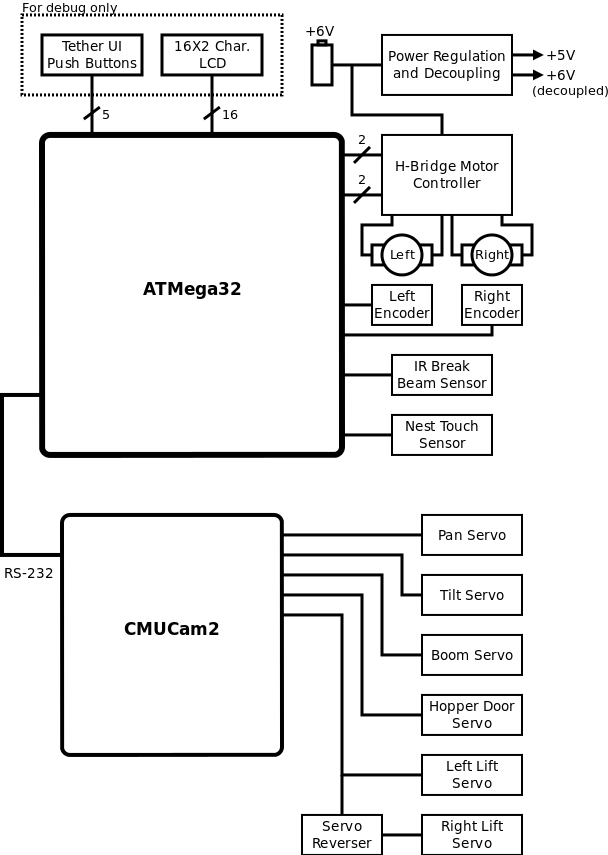
We opted to design and build our own power regulation and motor control circuitry over purchasing one of the more expensive off-the-shelf solutions. To ensure that we were not debugging software and electrical issues at the same time, we made sure to include robust regulation and decouple in the design. Our power sub-component power needs were:
Unregulated voltage was connected to the CMUcam2 (it had a built-in regulator) and to the motors. Although not ideal, connecting the motors to unregulated power meant we could save on cost by using a smaller, cheaper voltage regulator. We opted for a linear regulator to supply the +5V to the ATMega32 microcontroller.
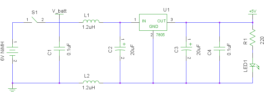
In the choice between a linear regulator and a switching regulator, a linear was chosen over a switching regulator for the following reasons:
Switching regulators are more efficient, however any efficiency gains would be dwarfed in comparison with the power demands of the unregulated components (DC motors and CMUcam2). The circuit diagram for our implementation is shown below:
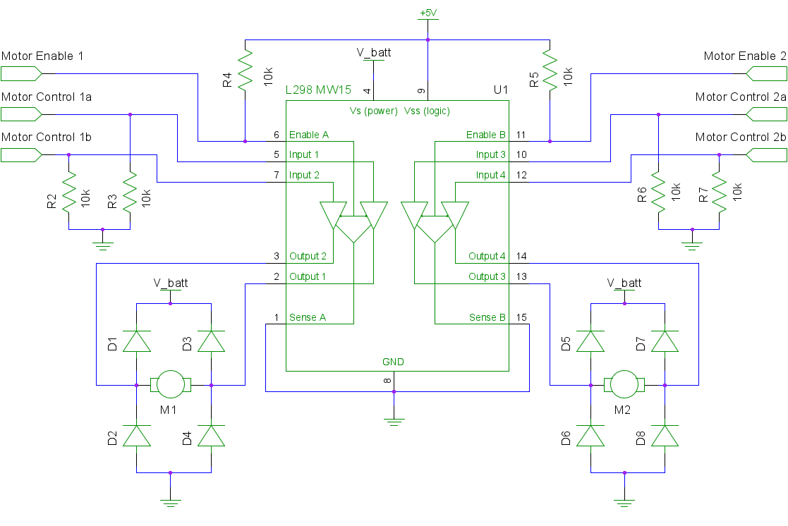
To control the motors via digital signal we used an H-bridge circuit. For added protection of the electronics from the back-EMF voltage of the motors, additional diodes were connected as shown in the schematic below.
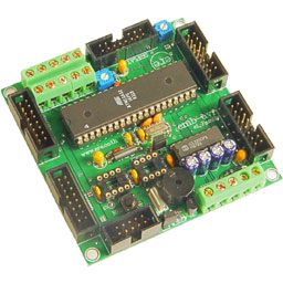
The power regulation and motor control circuits were fabricated together on a single board using a copper-plated board, etching solution, and a laser print out of the circuit layout. We made sure to use polarized headers for all the connections to avoid making any reverse polarity mistakes — though we still managed to make a couple!.
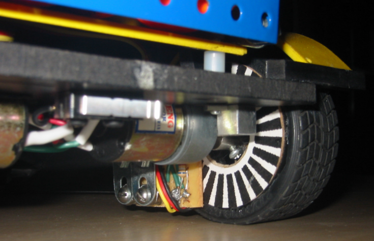
The maneuvers needed at junctions and for the bonus ball pick up sequences needed to be accurate and repeatable. To achieve this we use a simple differential drive system with encoders on each drive wheel. The encoders were made up of reflective IR sensors pointed at black and white patterned disks pasted to the inside edge of each drive wheel. [2]

The reflective IR sensors emit infrared light and measure the amount of infrared light that is reflected back with a photodiode. Since the white segments of the pattern reflect more light than the black segments, rotations of the wheel can be detected by thresholding the measured IR signal level. To guard against "chattering" when signals close to the threshold are applied a dual-threshold Schmitt trigger is needed. The precision of this wheel encoder system is equal to about one segment arc angle — 7.5° for a 48 segment pattern.
The P5587 reflective IR sensor package chosen for Caddy was designed for exactly this type of high contrast edge detection and so came with built in Schmitt triggers and a logic-level output that could be easily read by a GPIO input port on the microcontroller.
In order to capture ground balls, Caddy needed a way to detect when a ball was within the grasp of its lift mechanism.
We originally planned to use the centroid tracking feature of the camera since the camera would always be facing down for line tracking during the times it needed to detect ground balls. This turned out to be difficult mainly due to the limitations of the camera. When the camera is configured to track a black line both the glare from the overhead lighting and the randomly placed ground have the same effect on what the camera detects – a gap in the line. We tried to simply change modes whenever a gap was detected, determine if the gap was due to a glare or a due to a ball, and then act accordingly. Unfortunately, the CMUcam did not handle rapid mode and parameter changes well, taking too long to switch from one mode to another. This lead to a failure in our carefully tuned PID line tracking algorithm which relied on frequent, regular updates over time. We considered and experimented with some ways of solving this problem but none were the quick, elegant solution we were looking for.
With a fast approaching deadline, we opted for a quick, but less elegant, solution. We installed an IR break beam sensor looking across the front of the lift arm so that when the arm was down and fully open a ground ball would break the beam as is passed under the arm.
The mechanical design of Caddy required 6 servos:
This meant that the original plan to use the five servo control outputs of the CMUcam would be inadequate.
The following approaches were considered for accommodating the 6th servo output:
Searching the Internet, we found we were not the only ones to think of using a 555 timer to create a servo reverser. Using the well documented plans from C. Dane [1] we fabricated a board the size of a postage stamp.
For our our computing platform we chose an ATmega32 microcontroller from Atmel's 8-bit AVR line of microcontrollers because it was C-programmable with free open-source tools and because we had a readily available development board, the ERE EMBMega32.
To track the black electrical tape line, we implemented a proportional–integral–derivative (PID) controller. In PID theory, the output of a PID controller,  , is defined as:
![\[ c(t) = P_E e(t) + P_I \int e(t) dt + P_D \frac{de}{dt} \]](form_8.png)
Where  is some error function and
  ,
,  , and
, and  are adjustment coefficients for the observed error, the integrated error and the derivative of the error, respectively. We define our error term:
![\[ e(t) = \frac{dx}{dt} \]](form_9.png)
By substitution, we get:
![\[ c(t) = P_E \frac{dx}{dt} + P_I x(t) + P_D \frac{d^2x}{dt^2} \]](form_10.png)
Broken down and interpreted for the task of line tracking, these terms are:
 How fast are we drifting from the center line?
  How far are we from from the center line?
  How fast is the drift rate accelerating?
Provided that there is a way to measure or compute each of these terms, this is a more robust form of the equation because it eliminates the integral term which can cause problems due to accumulated error.
The figure below shows how the camera was used to measure  :
:
The drift rate is the slope of the black line with respect to the center line of the robot. For points  and
and  from the diagram above we define:
![\[ \frac{dx}{dt} = \frac{y_2-y_1}{x_2-x_1} \]](form_16.png)
And for point  with constant, measurable value for
  and for constant, measurable line center
![\[ x_3 = x_{center} - \frac{dx}{dt} (y_3 - y_1) + x_1; \]](form_28.png)
Lastly, by storing the previously computed value of  , we can compute the third term:
![\[ \frac{d^2x}{dt^2} = \frac{dx}{dt} - \frac{dx}{dt}_{previous} \]](form_25.png)
The coefficients for each of these terms were determined by trial and error using a tethered remote and stored persistently in EEPROM.
When turning our bot by a certain number of ticks, we experienced overshoot despite actively applying DC motor braking. We addressed the problem with the following software solution.
After turning for the desired number of ticks, we applied braking and counted the number of excess ticks that occurred from the instant braking was commanded. After a fixed delay, we drove the wheels in the opposite direction for that same number of ticks.
This worked well for the most part, however, with different battery charges, turn amounts, and turn types, the amount of time to brake was never the same. If we did not brake the motors for a long enough delay, our bot would stop counting excess ticks and begin to drive the motors in the opposite direction, too soon. With our unsophisticated encoders that cannot detect the direction of wheel motion this resulted in "reverse ticks" being counted before the wheel had actually started moving in the reverse direction.
While the locations of the ground balls were not known a priori, the map of the course was. We defined the course as a connected undirected graph with 42 nodes (vertices) as shown below. A node was placed at:
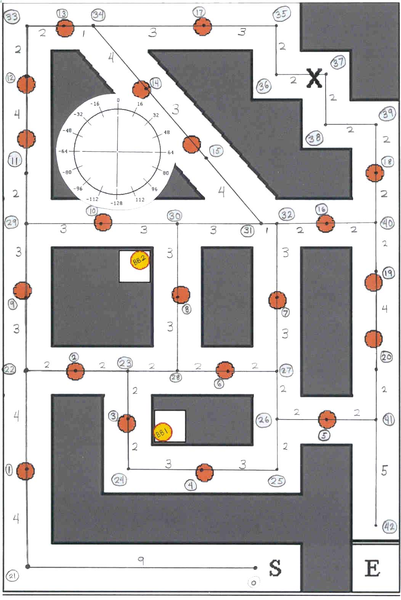
The software implementation of this graph was done using a C struct:
Each node defined the adjacent node numbers, directions, and distances to each adjacent node. Headings were defined in units of 8-bit binary radians or "brads". An 8-bit brad is 1/256 of a complete rotation. Brads are particularly useful in that they leverage the inherent rollover digital adders to automatically constrain the range of angular arithmetic operations to [0° 360°). Distances were stored using inches scaled by a factor of 1/6 since most node-to-node distances were multiples of 6 inches. This allowed all distances to be encoded in an 8-bit integer data type.
As an additional measure to conserve memory resources, information about the type of node was encoded in the node number:
SRAM memory was particularly limited on our ATMega32 platform, so to conserve it for other uses, the node list was stored in FLASH using a switch statement lookup table. This technique forces the constant values to be encoded in Load Program Memory (LPM) instruction words which are stored and accessed directly from FLASH.
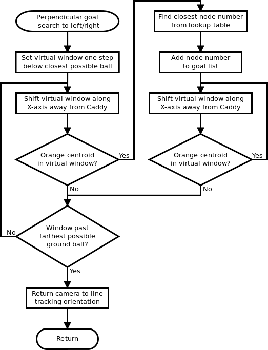
Except for a couple special cases, all ball detection was done at junctions with the tilt servo oriented vertically and the panning servo oriented at a fixed angle to the left or to the right. This covered all junctions in which a ground ball could be located down a perpendicular corridor to the left or right.
The ball detection algorithm was implemented using the built-in color tracking and virtual window features of the CMUcam. As with the line tracking, it was important that all the data processing intensive operations be done on the CMUcam processor in order to achieve low execution time.
At every junction, Caddy traversed all connected nodes in the graph extending to the left, for example. For any ground ball node encountered during this graph traversal that had not yet been checked, the node number was recorded along with distance away from the Caddy's current node location. If there was at least one unchecked ball node to the left, Caddy would orient the camera pan/tilt servos to look in that direction and use a sliding window algorithm to search for the ball.
As shown in the diagram below, the ball detection algorithm searched for the bottom of the ball by progressively moving a narrow image window through the image and using an upper and lower color intensity thresholds to determine if any orange pixels were within the image window.
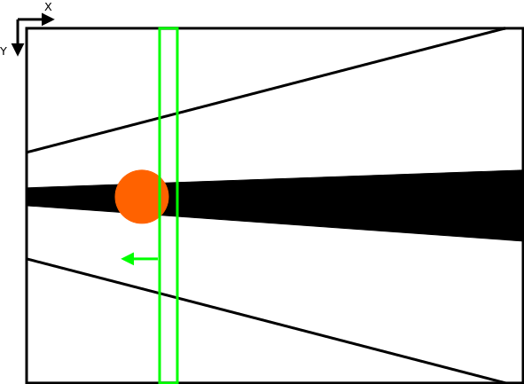
If an orange pixel was found, a look-up table was used to convert the the horizontal X coordinate of the image window to a physical distance away from the bot. This distance was then compared with the values in the unchecked ball list to find the most likely node number corresponding to the blob of orange pixels.
Since stopping to perform these ball searches added time to the run we made sure to mark any node that was "seen" during a ball search or physically crossed by Caddy as having been checked. Also, once the final ground ball was discovered all remaining unchecked nodes were marked as having been checked (by process of elimination). These optimizations ensured that Caddy only performed ball searches when necessary.
To optimize the computation time of the sliding window search algorithm, the window width was increased from 1 pixel to 4 pixels. We found that this gave sufficient resolution while providing a speedup of nearly 4.0. We also limited the far end of the sliding window range to cover just six inches past the farthest unchecked ball node since there was no point in search through parts of the image which we knew would not offer any new information. With these optimizations a typical ball search to the left or right took about 1 second.
The connected graph map of the arena and ball detection features described in the previous sections provided pieces of information needed for a path planning algorithm:
Now, every time a goal was added to the goal list (i.e. a ground ball was found), the path planning algorithm would compute the cost through all permutations of known goals starting from the current node and ending at nest node. This required two sub-algorithms:
The permutation algorithm proved to be more challenging than originally expected because the limited stack space of the ATmega32 precluded the use of a recursive permutation algorithm. With some research we found a simple iterative implementation in the GNU C++ Standard Template Library (STL). Adapting this templated code to C99 C code we had a solution for computing all permutations of any array of 8-bit values.
 1.8.1.2

